이미지 처리 작업은 데이터 변환을 수행하는 데 필요한 정보에 따라 세 가지 클래스로 나눌 수 있습니다. 가장 간단한 것부터 가장 복잡한 것까지 정렬하자면 다음과 같습니다:
- Point operation
- Neighborhood processing
- Geometrical transforms
Arithmetic operations
np.clip
픽셀 값에서 간단한 사칙연산을 통해 이미지를 변환할 수 있습니다. $y=x$ 값을 가지는 값에 128을 더하거나 빼면

다음과 같은 개형의 그래프를 얻을 수 있습니다. Python 에서는 numpy.clip 을 통해 구현할 수 있습니다.
np.clip 의 매개변수
np.clip(a, a_min, a_max)
- a: 값을 제한할 원래 numpy 배열
- a_min: 배열의 최소 허용 값
- a_max: 배열의 최대 허용 값
np.clip 사용예시
import numpy as np
import matplotlib.pyplot as plt
from PIL import Image

xray = Image.open('x-ray.png')
xray_np = np.array(xray).astype(np.float64)
# 보통 이미지는 uint8인데, 이대로 clip을 실행하면 오버플로우나 언더플로우가 발생할 수 있다.
# 꼭 float32나 float64로 변환하자.

xray_bright = np.clip(xray_np + 128, 0, 255).astype(np.uint8)
xray_dark = np.clip(xray_np - 128, 0, 255).astype(np.uint8)

plt.figure(figsize=(8, 5))

plt.subplot(1, 3, 1)
plt.imshow(xray_np, cmap='gray')
plt.axis('off')
plt.title('Original')

plt.subplot(1, 3, 2)
plt.imshow(xray_bright, cmap='gray')
plt.axis('off')
plt.title('Brighter image')

plt.subplot(1, 3, 3)
plt.imshow(xray_dark, cmap='gray')
plt.axis('off')
plt.title('Darker image')

plt.show()

Complements

간단한 연산을 통해 negative image 를 얻을 수 있습니다. Numpy array 의 최대값에 numpy array 를 빼는 방식입니다.
import numpy as np
import matplotlib.pyplot as plt
from PIL import Image

bb = np.array(Image.open('x-ray.png'))
# Negative np array
bc = np.max(bb) - bb

plt.figure()
plt.imshow(bc, cmap='gray')
plt.axis('off')
plt.show(block=False)
Histogram
픽셀 값과 이미지에서 해당 픽셀의 발생 빈도를 나타내는 그래프입니다. 좀 더 지능적인 방법으로 point processing 을 가능케 합니다. 확률 밀도 함수의 일종이라고 볼 수 있습니다. matplotlib 으로 히스토그램을 플로팅할 수 있습니다.
Histogram 구현
plt.hist(img.flatten(), bins=256, range=[0, 255], color='skyblue')
- img: 이미지의 numpy array
- flatten: 2D array를 1D vector 로 평탄화하는 메서드. flaten 은 2D array 복사본에 적용되는데, ravle()를 대신 사용하면 원본에도 영향을 미친다.
- bins: 데이터를 나눌 구간의 개수
- color: 막대 그래프의 색
import numpy as np
import matplotlib.pyplot as plt
from PIL import Image

xray = Image.open('x-ray.png')
xray_np = np.array(xray).astype(np.float64)

plt.figure()
plt.hist(xray_np.flatten(), bins=256, range=[0,255], color='red')

plt.show()

Histogram 의 분포를 보면 이미지의 명도와 대조의 정도를 알 수 있습니다. 개형이 왼쪽으로 쏠려있으면 어둡고, 오른쪽으로 쏠려있으면 밝은 이미지입니다. 그리고 좌우로 퍼져있을수록 contrast 가 높은 이미지고 모여있을수록 contrast 가 낮은 이미지입니다. Contrast 가 낮으면 이미지가 희뿌옇게 보입니다. Contrast 를 높이기 위해 piecewise linear function 을 통해 히스토그램을 좌우로 stretching 할 수 있습니다.
Stretching
Stretching with linear function

한 곳에 쏠려있는 gray values 를 좌우로 늘립니다. 푸른 박스 안을 봅시다. 5 ~ 9 까지의 원본 pixel value 가 2 ~ 14 범위의 output pixel values 로 stretching 됩니다.

- function: $j = m(i - i_{min}) + j_{min}$
- i: input pixel parameter
- j: output pixel parameter
- m: $(j_{max} - j_{min})/(i_{max} - i_{min})$
Stretching with linear function 구현
skimage.exposure.rescale_intensity(img, in_range=(a, b), out_range(c, d))
- img: 조정할 이미지 배열
- in_range: 입력 이미지의 강도 범위
- out_range: 출력 이미지의 강도 범위
import skimage.exposure as ex
import numpy as np
import matplotlib.pyplot as plt
from PIL import Image

t = np.array(Image.open('x-ray.png'))
t1 = ex.rescale_intensity(t, in_range=(0, 255), out_range(64, 191))
Stretching with Gamma value

1차 함수 형태로만 stretching 할 수 있는 것은 아닙니다. Gamma 값을 이용해 더 세밀한 stretching 이 가능합니다.
Gamma 가 1보다 작으면 이미지가 밝아지고, gamma가 1보다 크면 어두워집니다. 그래프의 개형을 보면 이해할 수 있습니다.
Stretching with Gamma value 구현
skimage.exposure.adjust_gamma(img, gamma)
- img: 조정할 이미지 배열
- gamma: Gamma value
t2 = ex.adjust_gamma(t, 0.5)
t3 = ex.adjust_gamma(t, 0.25)
Piecewise linear transformation
일부분만 stretching 할 수도 있습니다. 즉, 0부터 100은 40부터 100으로, 100부터 150은 100부터 220으로, 150부터 255는 220부터 255로 stretching 할 수 있다는 말입니다.
Piecewise linear transformation 구현
a = np.array([0, 100, 150, 255])
b = np.array([40, 100, 220, 255])

lin = np.interp(range(256), a, b)

t4 = np.zeros(t.shpae)
for i in range(256):
		idx = np.where(t == i)
		t4[idx] = lin[i]
Histogram Equalization

단 한번의 stretching을 사용할 때도 있지만, 여러 조합의 stretching 과정을 적용해서 좋은 이미지를 얻는 경우도 있습니다. Contrast stretch 의 각 과정을 일일이 직접 수행하는 것은 굉장히 번거롭습니다. 이것을 편하게 하기 위해 히스토그램을 사용해서 자동으로 contrast 를 조절할 수 있습니다. 이를 Histogram equalization 이라고 합니다. 이 때 사용하는 transformation function 은 정해져있습니다. 바로 CDF 입니다.
HE 의 transformation function 이 CDF 인 이유
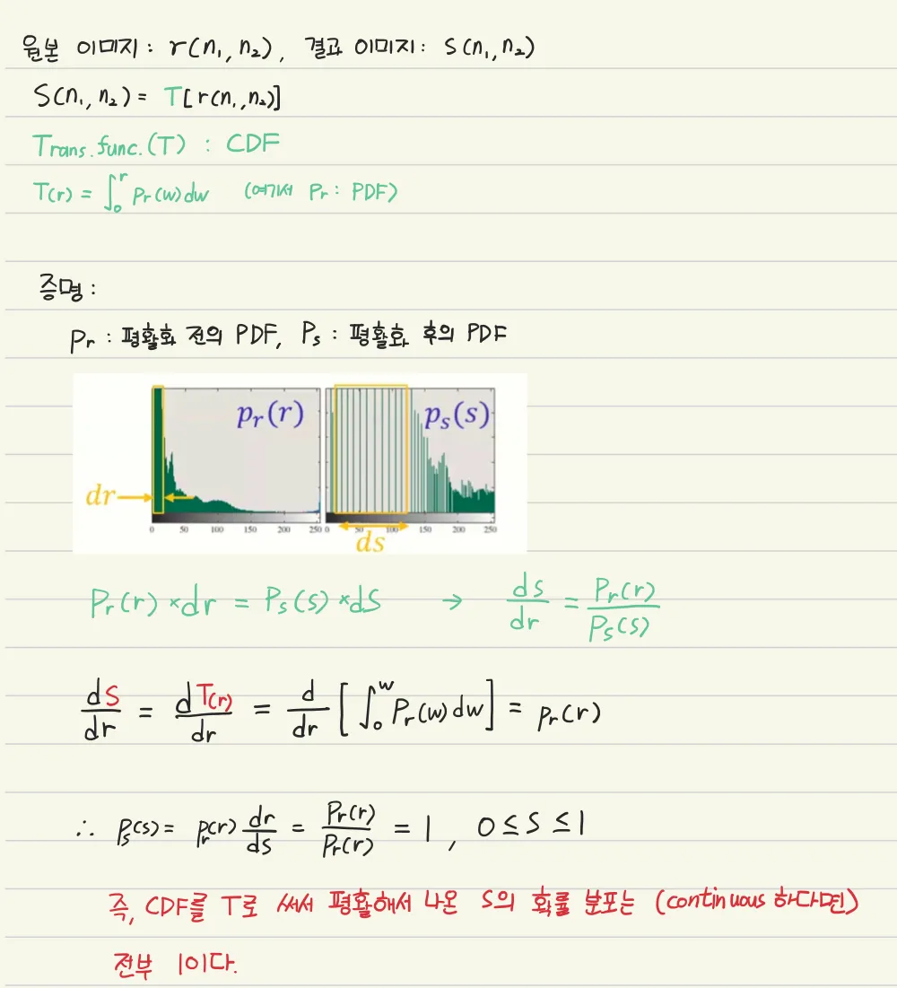
Discrete 한 환경에서도 CDF 로 평활화하면 continuous 환경과 정확하게 일치하지는 않지만 꽤나 근사한 결과를 얻을 수 있습니다.
HE 과정
- Input image 의 pr(r) 즉, 히스토그램을 구한다.
- 변환 함수 T(r) 로 사용할 CDF 를 계산하여 LUT 을 만든다.
- T(r) 을 이용해 input pixel value r 을 output pixel value s로 변환한다.
- Output image 의 적절한 위치에 s 를 입력한다.
HE 의 한계
- Transformation function 이 CDF 로 고정되어있다.
- 이미 contrast 가 좋은 이미지에서는 의미가 없다.
HE 구현
Equalization 을 할 때는 pixel values 가 0 ~ 1 로 정규화되어야 하고, histogram 을 만들어야 할 때는 다시 0 ~ 255 로 돌려야함을 잊으면 안됩니다.
import skimage.exposure as ex
import numpy as np
import matplotlib.pyplot as plt
from PIL import Image
from skimage.color import rgb2gray

gd = rgb2gray(np.array(Image.open('gdforce.jpeg')).astype(np.uint8))
equalized_gd = ex.equalize_hist(gd)

plt.figure(figsize=(14, 10))

plt.subplot(2, 2, 1)
plt.hist(gd.flatten() * 255, bins=256)
plt.title('Original GD Histogram')

plt.subplot(2, 2, 2)
plt.hist(equalized_gd.flatten() * 255, bins=256)
plt.title('Equalized GD Histogram')

plt.subplot(2, 2, 3)
plt.imshow(gd, cmap='gray')
plt.title('Original GD Image')
plt.axis('off')

plt.subplot(2, 2, 4)
plt.imshow(equalized_gd, cmap='gray')
plt.axis('off')
plt.title('Equalized GD Image')

plt.show()
더 좋은 이미지를 얻었다고 할 수는 없지만 적어도 contrast 는 확실히 좋아졌음을 확인할 수 있습니다.
'개발 > 의학영상처리' 카테고리의 다른 글
| 의학영상처리 Intro (3) | 2025.01.05 |
|---|